Authors:
(1) Albert Gu, Machine Learning Department, Carnegie Mellon University and with equal contribution;
(2) Tri Dao, Department of Computer Science, Princeton University and with equal contribution.
Table of Links
3 Selective State Space Models and 3.1 Motivation: Selection as a Means of Compression
3.2 Improving SSMs with Selection
3.3 Efficient Implementation of Selective SSMs
3.4 A Simplified SSM Architecture
3.5 Properties of Selection Mechanisms
4 Empirical Evaluation and 4.1 Synthetic Tasks
4.4 Audio Modeling and Generation
4.5 Speed and Memory Benchmarks
A Discussion: Selection Mechanism
D Hardware-aware Algorithm For Selective SSMs
E Experimental Details and Additional Results
4.6 Model Ablations
We perform a series of detailed ablations on components of our model, focusing on the setting of language modeling with size ≈ 350M models at Chinchilla token counts (same setting as Figure 4).
4.6.1 Architecture
Table 6 investigates the effects of the architecture (block) and its inner SSM layer (Figure 3). We find that
• Among previous non-selective (LTI) SSMs, which are equivalent to global convolutions, performance is very similar.
• Replacing the complex-valued S4 variant from previous work with a real-valued one does not affect performance much, suggesting that (at least for LM) real-valued SSMs may be a better choice when accounting for hardware efficiency.
• Replacing any of these with a selective SSM (S6) significantly improves performance, validating the motivation of Section 3.
• The Mamba architecture performs similarly to the H3 architecture (and seems slightly better when using a selective layer).
We also investigate interleaving the Mamba block with other blocks such as MLP (a traditional architecture) MHA (a hybrid attention architecture) in Appendix E.2.2.
4.6.2 Selective SSM
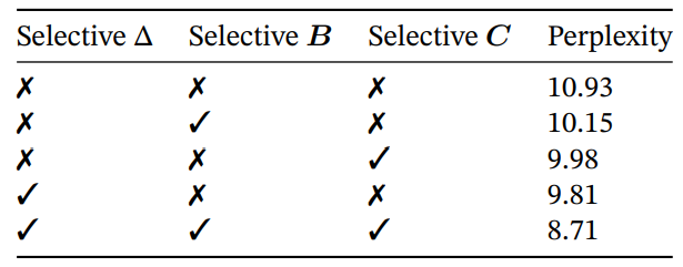
Table 7 ablates the selective SSM layer by considering different combinations of selective ∆, B, and C parameters (Algorithm 2), showing that ∆ is the most important parameter due to its connection to RNN gating (Theorem 1).
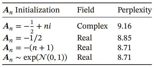
Table 8 considers different initializations of the SSM, which have been shown to make a large difference in some data modalities and settings (Gu, Goel, and Ré 2022; Gu, Gupta, et al. 2022). On language modeling, we find that simpler real-valued diagonal initializations (S4D-Real, row 3) instead of more standard complex-valued parameterizations (S4D-Lin, row 1) perform better. Random initializations also work well, consistent with findings from prior work (Mehta et al. 2023).
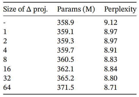
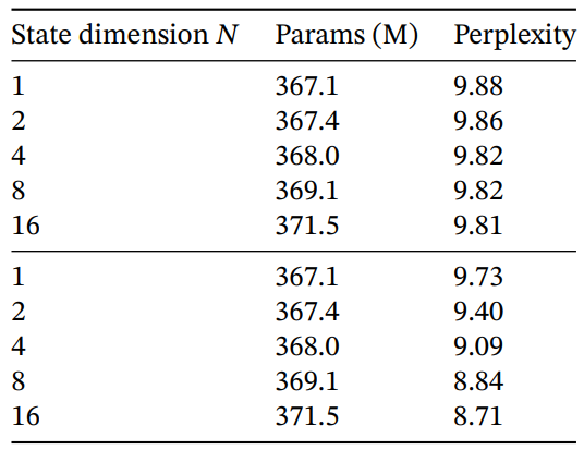
Table 9 and Table 10 consider varying the dimension of the ∆ and (B, C) projections respectively. Changing them from static to selective provides the most benefit, while increasing the dimensions further generally improves performance modestly with a small increase in parameter count.
Of particular note is the dramatic improvement of the selective SSM when the state size N is increased, with over a 1.0 perplexity improvement for a cost of only 1% additional parameters. This validates our core motivation in Sections 3.1 and 3.3.


This paper is available on arxiv under CC BY 4.0 DEED license.

