An Overview of the Data-Loader Landscape: Experimental Setup

Table of Links

• Abstract and Intro
• Dataloaders
• Experimental Setup
• Numerical Results
• Discussion
• Related Work
• Conclusion, Acknowledgments, and References
• A. Numerical Results Cont.

3. EXPERIMENTAL SETUP

Several libraries and datasets were selected to compare their features and performance. Even though an effort was made to be as comprehensible as possible, the field of data loading is constantly evolving and new libraries and releases are added every day. In this regard, we expect the following list to provide a good overview of the current capabilities of dataloaders, without necessarily claiming or finding the overall best (which would probably change from the time of writing to the time of publication). We make all the source code of the experiments available to the public and expect results to be fully reproducible.

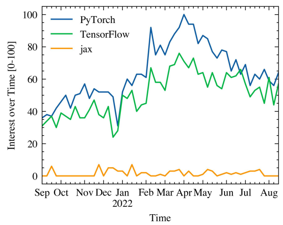
We selected seven libraries to perform our experiments: PyTorch (Paszke et al., 2019), Torchdata (TorchData, 2021), Hub (Team, 2022a), FFCV (Leclerc et al., 2022), Webdatasets (Webdataset, 2013), Squirrel (Team, 2022b), and Deep Lake (Hambardzumyan et al., 2022). One interesting thing that we discovered is that not all libraries support the same features. For example, we could not run FFCV with a dataset hosted in an S3 bucket to perform our remote experiments. As we mentioned in Section 1, we run all our experiments in PyTorch. We considered reproducing the experiments in other popular machine learning frameworks but we decided against the idea since the second candidate would have been Tensorflow, but there are rumors that Google is moving away from it in favor of JAX. Figure 1 depicts the popularity of different ML frameworks in the last 12 months.

3.1 Datasets

Regarding the datasets, we initially opted for two classical datasets to support two different learning tasks: CIFAR-10 (Krizhevsky et al., 2009) for image classification, and CoCo (Lin et al., 2014) for object detection. While performing some experiments, we observed strange behavior (libraries performing better than expected) that could be explained by

CIFAR-10 fitting into memory[2]. For this reason, we built a third dataset named RANDOM, consisting of randomly generated colour images of size 256 by 256 pixels and a random class out of 20. This third dataset contains 45000 images for training, 5000 for validation, and 500 for testing, and it is considerably larger than CIFAR-10.

We used the same transformations for all libraries to make the benchmarks comparable. The only exception was FFCV, which has its own implementation of the different transformations. For image classification the transformation stack consisted of the following: Random Horizontal Flip, Normalization, Cutout, Transform into Tensor.

For object detection, we relied mostly on Albumentations’ (Buslaev et al., 2020) implementation of transformations. The stack looked as follows: Random Sized Crop, Random Horizontal Flip, Normalization, Transform into Tensor. These transformations apply to both, images and bounding boxes.

3.2 Experiment Variants

When possible, we hosted the dataset locally and in an S3- equivalent bucket. This enabled us to assess the slowdown resulting from training from a stream of data over the network. We will provide a detailed description of the training setting in Section 4.

Given that the most intensive training jobs involve using more than one GPU, whenever possible we also ran the same experiments in an environment with multiple GPU units. Because at the time of running the experiments not all libraries had the full support of PyTorch Lightning, we decided to implement the multi-GPU using the Distributed Data Parallel (DDP) (Li et al., 2020) library from PyTorch.

For some machine learning projects, we might need access only to a subset of a larger dataset. For those cases, having the ability to quickly filter the required data points without having to iterate over the whole dataset can drastically reduce the total training time. Some libraries allow filtering based on certain features, such as the class (for image classification tasks). We explored the gain (or loss) in speed for using the filtering method provided by the library (in case it offered one) versus not filtering at all. Whenever the library did not offer a filtering method, we implemented them naively, i.e., scanning the whole dataset and keeping only those elements that match the specified condition. Fast filtering is not necessarily trivial to implement as it requires an index-like additional structure to be maintained to avoid iterating over all samples.

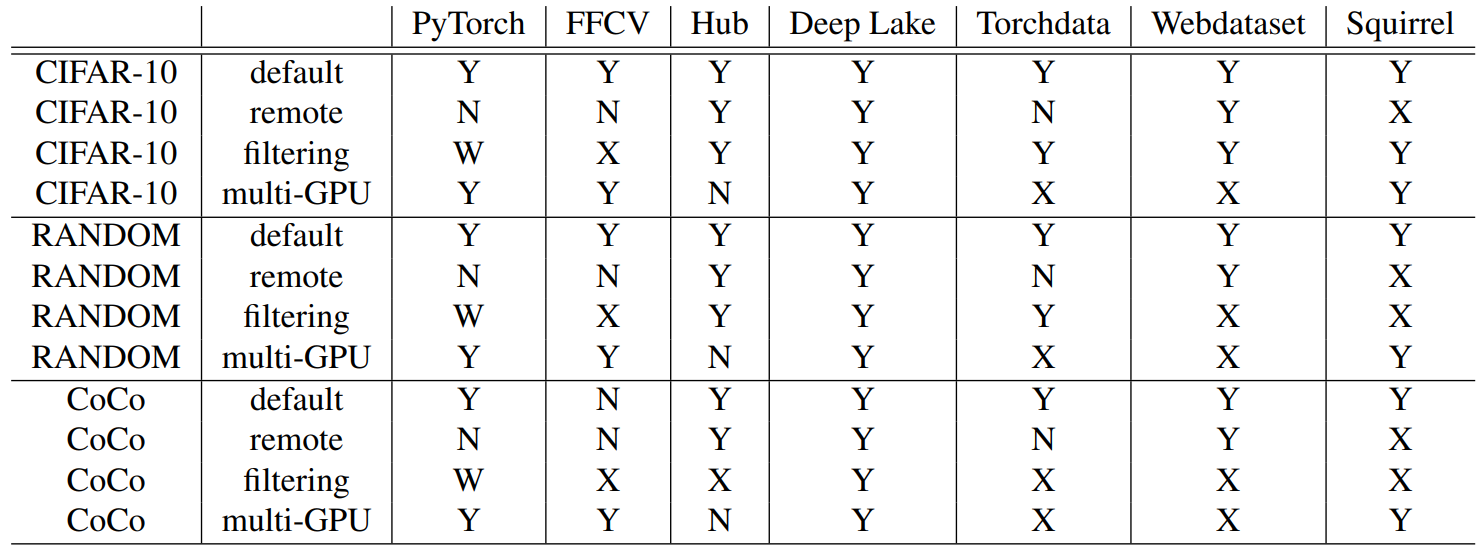
Finally, Table 1 specifies the compatibility of the different libraries with the different experiments and datasets we explored in this paper.

3.3 Metrics

Our main priority when building the experiments was to find an objective metric that would allow us to compare all the different libraries in a way that was sound.

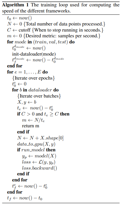
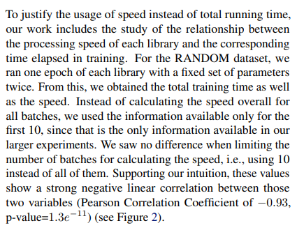
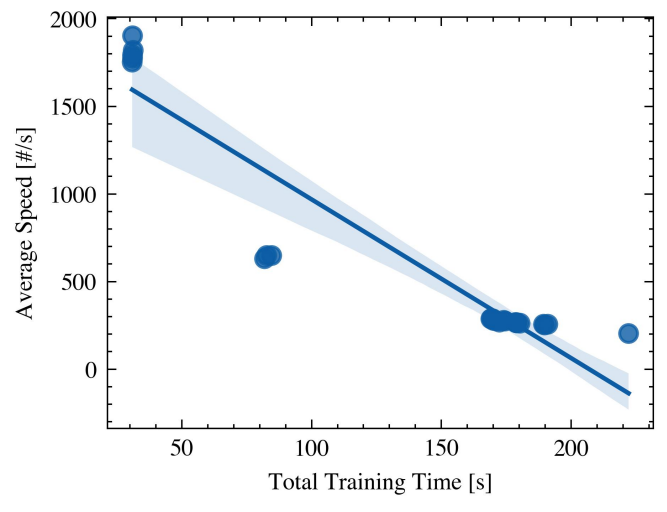
The ideal metric would have been the total running time of the training job since this is what we have to wait and pay for. Unfortunately, that would have greatly limited the number of experiments we could ran. After careful consideration, we opted for the number of processed data points (images) per second, a result backed by our numerical experiments. We consider two variants of this metric: one in which we use the ML model to train and we perform backpropagation and one in which we do not use the ML model and only iterate over the samples, copying them to GPU. The difference between the two metrics can be appreciated from the pseudo-code of the training loop in Algorithm 1, where m denotes the speed variable. We also collected the total running time[3] and the time it took for the dataloaders to be initialized. The latter was motivated by the fact that some of the libraries might perform expensive computations upfront to increase their speed while training. We also ended up performing a warm-up for calculating the speed. This is discussed further in Subsection 3.5.

3.4 Correlation between speed and running time

3.5 A closer look into running times

To increase our understanding of the inner mechanisms in each library, we decided to inspect for a single run how long it took to execute each batch as well as to initialize the dataloader. Figure 3 depicts for a single combination of parameters [4], the time taken by each library in the steps described by Algorithm 1. All these experiments involved a cutoff after 10 batches.

Interestingly, the first batch takes a considerable time longer than the others. This can be explained as follows: since most dataloaders rely on lazy loading data at this point, future calls will benefit from pre-fetching, data already in memory, and parallelization (doing things while the GPU is busy doing computations).

The size of the bands 1 to 9 provides the best indication of how well each library scales since the time taken on a

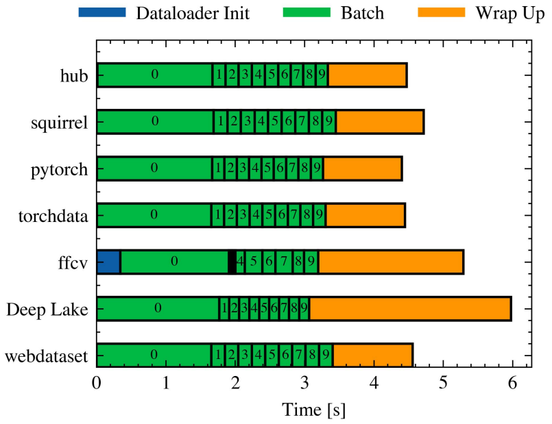
large dataset grows linearly with that width. We can observe that most libraries have a uniform width, with Deep Lake being the shortest (the fastest). On the other hand, the only library that shows non-homogeneous widths is FFCV, where the bands 1 to 3 are so thin that they cannot be seen in the image.

The wrap-up period takes about the same time for all libraries except for FFCV and Deep Lake, which take considerably longer. The time spent wrapping up depends mostly on the model and is not necessarily indicative of how well each library scales.

Based on this figure, we decided to perform a warm-up when computing the speed. This translates into ignoring the time taken by the first batch in all speed calculations.

[2] This is often something desirable and expected in some of the reviews literature, but we found it not to be the case in several practical applications involving small teams and in-house workstations.

[3] This is the time from the start of the simulation until the cutoff, which in practice was often only 10 batches.

[4] RANDOM dataset, single GPU, 0 workers, batch size 64